1. Overview
The parameter server aims for high-performance distributed machine learning applications. In this framework, multiple nodes runs over multiple machines to solve machine learning problems. There are often a single schedule node, and several worker and servers nodes.
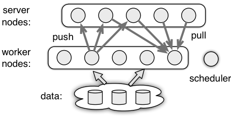
- Worker. A worker node performs the main computations such as reading the data and
computing the gradient. It communicates with the server nodes via
pushandpull. For example, it pushes the computed gradient to the servers, or pulls the recent model from them. - Server. A server node maintains and updates the model weights. Each node maintains only a part of the model.
- Scheduler. The scheduler node monitors the aliveness of other nodes. It can be also used to send control signals to other nodes and collect their progress.
1.1. Distributed Optimization
Assume we are going to solve the following
where (yi, xi) are example pairs and w is the weight.
We consider solve the above problem by minibatch stochastic gradient descent (SGD) with batch size b. At time t, this algorithm first randomly picks up b examples, and then updates the weight w by
We give two examples to illusrate the basic idea of how to implement a distributed optimization algorithm in ps-lite.
1.1.1. Asynchronous SGD
In the first example, we extend SGD into asynchronous SGD. We let the servers maintain w, where server k gets the k-th segment of w, denoted by wk<\sub>. Once received gradient from a worker, the server k will update the weight it maintained:
t = 0;
while (Received(&grad)) {
  w_k -= eta(t) * grad;
  t++;
}
where the function received returns if received gradient from any worker
node, and eta returns the learning rate at time t.
While for a worker, each time it dose four things
Read(&X, &Y);  // read a minibatch X and Y
Pull(&w);      // pull the recent weight from the servers
ComputeGrad(X, Y, w, &grad);  // compute the gradient
Push(grad);    // push the gradients to the servers
where ps-lite will provide function push and pull which will communicate
with servers with the right part of data.
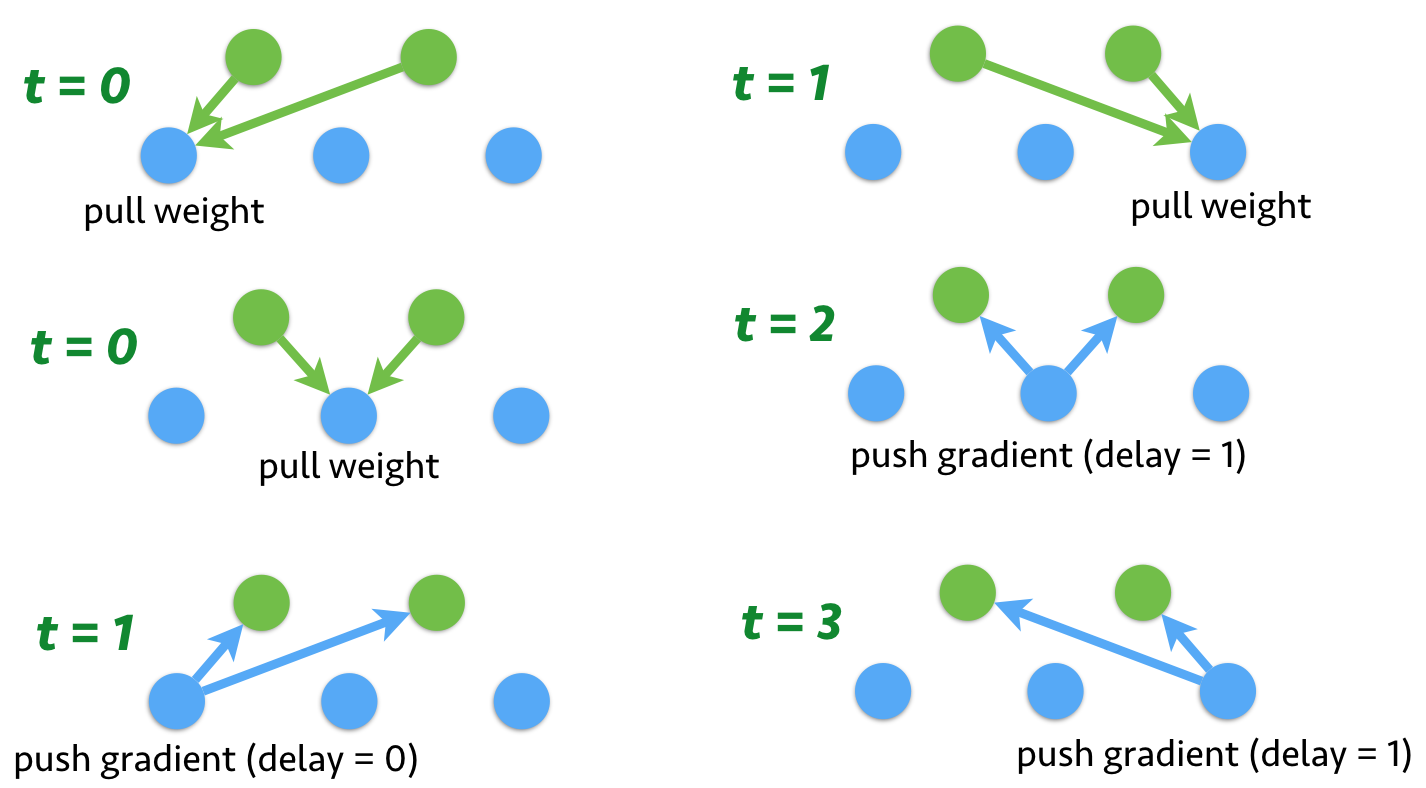
Note that asynchronous SGD is semantically different the single machine version. Since there is no communication between workers, so it is possible that the weight is updated while one worker is calculating the gradients. In other words, each worker may used the delayed weights. The following figure shows the communication with 2 server nodes and 3 worker nodes.
1.1.2. Synchronized SGD
Different to the asynchronous version, now we consider a synchronized version, which is semantically identical to the single machine algorithm. We use the scheduler to manage the data synchronization
for (t = 0, t < num_iteration; ++t) {
  for (i = 0; i < num_worker; ++i) {
     IssueComputeGrad(i, t);
  }
  for (i = 0; i < num_server; ++i) {
     IssueUpdateWeight(i, t);
  }
  WaitAllFinished();
}
where IssueComputeGrad and IssueUpdateWeight issue commands to worker and
servers, while WaitAllFinished wait until all issued commands are finished.
When worker received a command, it executes the following function,
ExecComputeGrad(i, t) {
   Read(&X, &Y);  // read minibatch with b / num_workers examples
   Pull(&w);      // pull the recent weight from the servers
   ComputeGrad(X, Y, w, &grad);  // compute the gradient
   Push(grad);    // push the gradients to the servers
}
which is almost identical to asynchronous SGD but only b/num_workers examples are processed each time.
While for a server node, it has an additional aggregation step comparing to asynchronous SGD
ExecUpdateWeight(i, t) {
   for (j = 0; j < num_workers; ++j) {
      Receive(&grad);
      aggregated_grad += grad;
   }
   w_i -= eta(t) * aggregated_grad;
}
1.1.3. Which one to use?
Comparing to a single machine algorithm, the distributed algorithms have two additional costs, one is the data communication cost, namely sending data over the network; the other one is synchronization cost due to the imperfect load balance and performance variance cross machines. These two costs may dominate the performance for large scale applications with hundreds of machines and terabytes of data.
Assume denotations:
| \({f}\) | convex function |
| \({n}\) | number of examples |
| \({m}\) | number of workers |
| \({b}\) | minibatch size |
| \({\tau}\) | maximal delay |
| \(T_{\text{comm}}\) | data communication overhead of one minibatch |
| \(T_{\text{sync}}\) | synchronization overhead |
The trade-offs are summarized by
| SGD | slowdown of convergence | additional overhead |
|---|---|---|
| synchronized | \(\sqrt{b}\) | \(\frac {n}b (T_{\text{comm}} + T_{\textrm{sync}})\) |
| asynchronous | \(\sqrt{b\tau}\) | \(\frac n{mb} T_{\textrm{comm}}\) |
What we can see are
- the minibatch size trade-offs the convergence and communication cost
- the maximal allowed delay trade-offs the convergence and synchronization cost. In synchronized SGD, we have τ=0 and therefore it suffers a large synchronization cost. While asynchronous SGD uses an infinite τ to eliminate this cost. In practice, an infinite τ is unlikely happens. But we also place a upper bound of τ to guarantee the convergence with some synchronization costs.
1.2. Further Reads
Distributed optimization algorithm is an active research topic these years. To name some of them
- Dean, NIPS‘13, Li, OSDI‘14 The parameter server architecture
- Langford, NIPS‘09, Agarwal, NIPS‘11 theoretical convergence of asynchronous SGD
- Li, NIPS‘14 trade-offs with bounded maximal delays τ
- Li, KDD‘14 improves the convergence rate with large minibatch size b
- Sra, AISTATS‘16 asynchronous SGD adaptive to the actually delay rather than the worst maximal delay
- Li, WSDM‘16 practical considerations for asynchronous SGD with the parameter server
- Chen, LearningSys‘16 synchronized SGD for deep learning.